The Vlookup function (finding an exact match):
Building the function step by step:
1. Type the following code: =vlookup(
2. Type the address of the cell containing the value that you wish to look for in the table.
3. Type the range of the table to look inside, (or better: Name the table before starting with the function, and type now its name). Remember: don’t include the table’s heading row.
4. Type the column number from which you want to retrieve the result.
5. Type the word FALSE which means: “Please find me exactly the value of the cell mentioned in step 2. (Don’t round it down to the closest match)”.
6. Close the bracket and hit the [Enter] key.
Note: The function will always look for the value mentioned on step 2 only on the first column (the utmost left column) of the table.
Vlookup Examples:
Let’s assume you are using the following Excel worksheet: (You can download it here)
Let’s assume you are using the following Excel worksheet: (You can download it here)
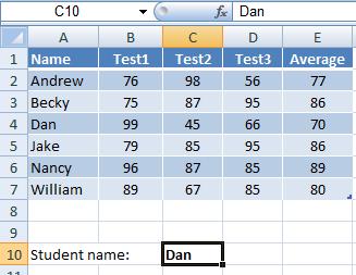
=vlookup(C10,A2:E7,2,FALSE)
In words: Look for the value in cell C10 inside table located at
A2:E7, and retrieve me the value on the 2’nd column. Please find me
exactly what’s in cell C10.
The value of the above formula will be: 99 (on Dan’s row, the second column).
The value of the above formula will be: 99 (on Dan’s row, the second column).
Copying and replicating the function
If you plan on copying the vlookup function, either by “copy” and “paste” or by dragging it with the fill handle, make sure to set the table’s address with fixed reference (e.g. $A$2:$E$7), but it would be better instead to name the table, as in the following example.
You can name the range A2:E7 by selecting it, and typing the name in the name box.
Let’s assume you named it studentsTable (spaces are not allowed, but you may use underscores).
=vlookup(c10,studentsTable,3,false)
In words: Look for the value in cell C10 inside studentsTable,
and retrieve the value from the table’s 3’rd column. Please find me
exactly what’s in cell C10.
The value of the above function will be: 45 (on Dan’s row, the value in the third column of the table).
The value of the above function will be: 45 (on Dan’s row, the value in the third column of the table).
Troubleshoot (advanced usage with more functions)
If the vlookup doesn’t find a match, it will write the following code: #N/A.
You can overcome this code, and set what do display in case it doesn’t find a value by using the IF function with the ISNA() function. Look at the following example:
If the vlookup doesn’t find a match, it will write the following code: #N/A.
You can overcome this code, and set what do display in case it doesn’t find a value by using the IF function with the ISNA() function. Look at the following example:
=if(isna(vlookup(c10,studentsTable,3,false)),”didn’t find any match”, vlookup(c10,studentsTable,3,false))
In words: if the vlookup function gives us the #N/A code, then write “didn’t find any match”, else compute the vlookup function.
Explanation:
The 3 parts of the above IF function are:
1. isna(vlookup(c10,studentsTable,3,false))
2. “didn’t find any match”
3. vlookup(c10,studentsTable,3,false)
The first part is a condition, which says: Does the vlookup function gives us the #N/A code?
If it does, write “didn’t find any match”, otherwise compute the vlookup function.
Tip:
Instead of the part “didn’t find any match”, you can put only double quotation marks “” which will leave the cell empty in case no match is found:
=if(isna(vlookup(c10,studentsTable,3,false)),””, vlookup(c10, studentsTable,3,false))
or let it retrieve the value 0 in case of no match:
=if(isna(vlookup(c10,studentsTable,3,false)),0, vlookup(c10, studentsTable,3,false))
The Vlookup function - closest match
Building the function step by step:
This is exactly the same process as building the vlookup with exact match, but with the following difference: Instead of writing FALSE at the end of the function, write TRUE.
Example:
Let’s assume you have the following worksheet, and the table is named “sales_table”:
This is exactly the same process as building the vlookup with exact match, but with the following difference: Instead of writing FALSE at the end of the function, write TRUE.
Example:
Let’s assume you have the following worksheet, and the table is named “sales_table”:
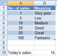
=vlookup(B10,sales_table,2,true)
In words: find me the value of cell B10 inside the first column
of sales_table, and retrieve me the value next to it from the table’s
second column. If you don’t find the value, relate to the closest
smaller value you can find.
Hence, the value 14 doesn’t appear on the first column of the table, so the function will relate to the value 10 which is the closest smaller value, and retrieve the word “medium” from the second column.
If the value of cell B10 was changed to 90, the vlookup would return us the word “Great” (the closest smaller match it finds would be 50).
Getting Rid of the Vlookup #N/A Error Code
When the vlookup function doesn’t find the value inside the range
specified, it will write the #N/A code, meaning “Not Available”.
To get rid of this error code, you can put the vlookup inside an IF function together with the ISNA function in the following format:
To get rid of this error code, you can put the vlookup inside an IF function together with the ISNA function in the following format:
=If (isna (vlookup(blabla)) , “”, vlookup(blabla))
In words:
If the vlookup function is N/A, then leave the cell blank, otherwise perform the vlookup function.
(It is recommended that you be familiar with the If Statement before you proceed.)
An Example (taken from the related video):
=If(isna(vlookup(D9,oldList,2,false)),””,vlookup(D9,oldList,2,false))
(Note the double parenthesis after the word “false” in both of its occurrences)
Let’s cut the above function into three parts, and examine them one by one:
First part:
=If(isna(vlookup(D9,oldList,2,false)),
In words:
If the function vlookup(D9,oldList,2,false) gives N/A - (this will happen if it didn’t find the value of cell D9 inside oldList),
Second part:
If the function vlookup(D9,oldList,2,false) gives N/A - (this will happen if it didn’t find the value of cell D9 inside oldList),
Second part:
“”,
In words:
Then leave the cell blank (double quotation marks mean “blank”)
Third part:
Then leave the cell blank (double quotation marks mean “blank”)
Third part:
vlookup(D9,oldList,2,false))
In words:
Otherwise perform the vlookup as usual.
No comments:
Post a Comment